
PID Controller Guide for Building Automation
A PID controller is one of the basic building blocks of building automation. It is used when a system has a measured value, a target value and an actuator that can change the process. Typical examples are supply air temperature controlled with a heating or cooling valve, duct pressure controlled with a variable speed fan, heating water temperature controlled with a valve, and room temperature controlled with a modulating or pulsed heating output.
The purpose of PID control is simple even though the terminology can make it look complicated. The controller compares the setpoint with the measured value, calculates the difference between them, and changes its output so that the measurement moves toward the setpoint. What makes PID useful is that it can do this continuously while the load changes. A heating valve can therefore settle at 18%, 47% or 83% instead of only switching fully open and fully closed.
In practice, the difficult part is not understanding that the controller should increase or decrease its output. The difficult part is deciding how strongly it should react, how quickly it should remove a remaining error, how much it should react to the rate of change, and how the tuning must change when the physical process is faster, slower or has more delay. The same PI settings that work well for a duct pressure loop can be completely unsuitable for room temperature control.
This guide explains PID control from the point of view of building automation commissioning and programming. It starts with the actual process behavior, then explains P, I and D, proportional band, 1/P, 1/I and 1/D coefficient forms, output limits, integral windup, sampling time, pulse outputs and practical tuning. The interactive examples use simplified process models so that the effect of each parameter can be seen directly.
PID parameter names are not standardized between all controller manufacturers. A value called P can mean proportional gain in one controller and proportional band in another. I may mean integral gain, integral time or an integral divisor. D may mean derivative gain, derivative time or another implementation-specific value. Always check the equation, units and controller documentation before copying tuning values from one system to another.
The first simulator intentionally starts with aggressive PI tuning. Change the proportional band and integral time until the water temperature reaches the setpoint without excessive overshoot or continuous oscillation. Apply a load disturbance after the loop has settled and watch whether the controller recovers. You can also switch the parameter view from proportional band and time values to the equivalent reciprocal coefficients used by the simulator.
1. Why PID control is used
A simple thermostat can control a process by switching an output on when the measurement is below the setpoint and switching it off when the measurement is above the setpoint. This is often called two-position or on/off control. It works well when the process can tolerate a repeating temperature swing and when the actuator is designed for switching. A domestic refrigerator is an obvious example. The compressor does not need to run at exactly 37.4% output to maintain temperature.
Many building automation processes benefit from smoother control. If a supply air temperature controller opened a heating valve fully every time the temperature was slightly low and closed it fully every time the temperature was slightly high, the supply temperature would move around the setpoint and the valve would make unnecessary full-stroke movements. A variable speed fan controlled in the same way would repeatedly accelerate and decelerate instead of finding the speed required to maintain duct pressure.
A PI or PID controller allows the output to take any value inside its configured range. If the process requires 43% valve opening to maintain 60 °C at the current load, the controller can remain close to 43%. If the load increases and 57% is required, the controller moves toward 57%. The output is therefore continuously adjusted according to the measured error and the history of the process.
The objective is not simply to make the measured value touch the setpoint once. A useful control loop should normally reach the setpoint in a reasonable time, reject normal disturbances, avoid sustained oscillation, avoid unnecessary actuator movement and remain stable across the operating range. Good tuning is therefore a compromise between speed and stability.
PID control is widely used in HVAC for supply air temperature, heating and cooling water temperature, duct pressure, differential pressure, room pressure, humidity and many other continuously controlled values. Many of these loops use PI control rather than full PID because the integral term removes steady-state error while derivative action is often unnecessary for slow and noisy HVAC measurements.
2. The parts of a closed control loop
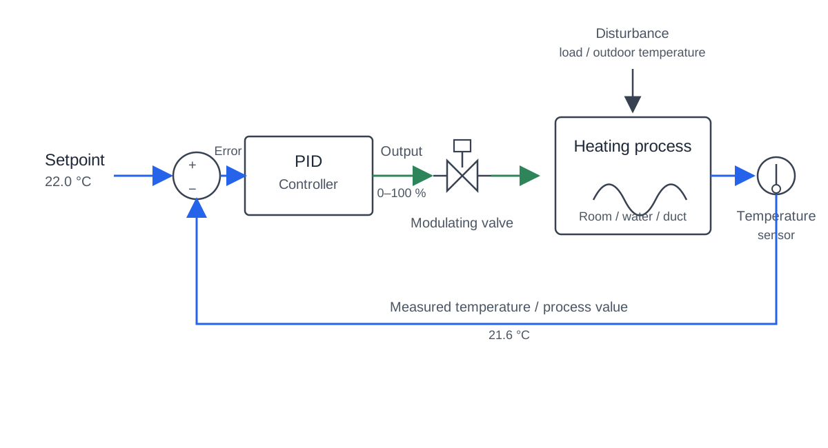
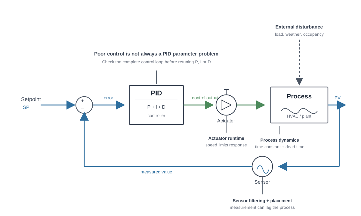
A controller cannot regulate anything by itself. It is one part of a complete closed loop that includes the setpoint, measurement, controller, actuator and physical process. When troubleshooting bad control, each of these parts has to be considered because poor sensor placement, a slow actuator or an oversized valve can produce a bad trend even when the PID calculation is correct.
The common terms are SP for setpoint, PV for process value or measured value, error for the difference between them, and output for the controller command. For a heating loop it is convenient to define the error as SP - PV. If the setpoint is 60 °C and the measured value is 55 °C, the error is +5 K. The controller then needs to increase heating demand. If the measurement rises above the setpoint, the error becomes negative and the controller needs to reduce heating demand.
A disturbance is something that changes the process without being commanded by the controller. In a heating water loop, an increase in water flow may increase the heating load and pull the controlled temperature down. In a room, an open window may increase heat loss. In a pressure loop, dampers opening in the duct system may reduce pressure. A well-tuned loop should recover from these disturbances without becoming unstable.
| Term | Meaning | Example |
|---|---|---|
| SP | Setpoint | 60 °C |
| PV | Process value | 55 °C |
| Error | SP - PV | +5 K |
| Controller output | Requested actuator command | 68% |
| Actuator | Device that changes the process | Heating valve |
| Process | Physical system being controlled | Water heating loop |
| Disturbance | External change in load | Increased water flow |
3. Controller direction must be correct first
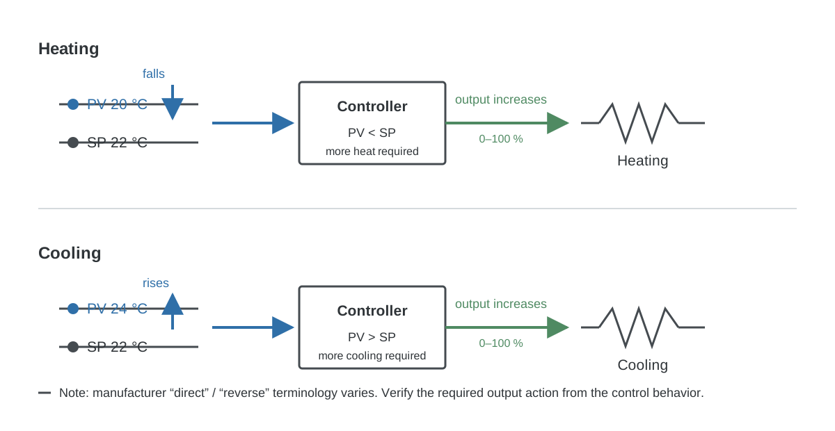
Before tuning P, I or D, verify that the output moves in the correct direction. In a heating loop, a falling temperature normally needs more heating output. In a cooling loop, a rising temperature normally needs more cooling output. A pressure controller may need more fan speed when measured pressure falls. A bypass damper controller may have the opposite actuator direction depending on how the damper is installed and how the signal is scaled.
Manufacturers use terms such as direct acting, reverse acting, heating action, cooling action, positive action and negative action, but these labels are not completely consistent between products. The safe commissioning method is to ignore the label for a moment and verify the physical behavior. Create a small error and confirm that the controller output moves in the direction that reduces that error. If a low heating temperature makes the heating valve close further, no amount of tuning will fix the loop.
4. Proportional control: what P actually does
The proportional term reacts to the error that exists right now. If the measurement is far from the setpoint, the proportional response is large. If the measurement is close to the setpoint, the proportional response is small. If the measurement is exactly at the setpoint, the proportional contribution is zero unless the controller implementation includes a separate bias or operating point.
There are two common ways to describe proportional action. A mathematical controller often uses proportional gain, usually written as Kp. A building automation controller often uses a proportional band, sometimes called P-band. These describe the same basic relationship from opposite directions. A larger gain gives a stronger response. A larger proportional band gives a weaker response.
For a controller whose output is normalized from 0 to 100%, the proportional-band form is easy to understand:
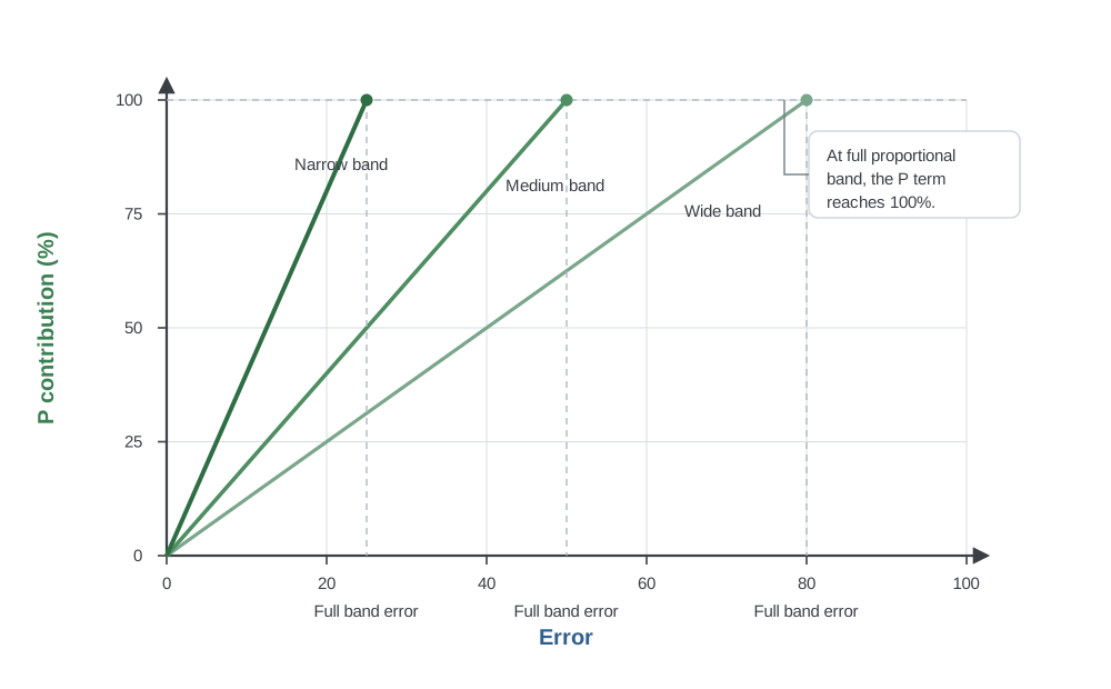
P contribution = error / proportional band x 100%
If the proportional band is 10 K and the error is 2 K, the proportional term requests a 20% change of the full controller output range. If the error is 5 K, it requests 50%. If the error reaches 10 K, the proportional contribution reaches 100%.
This is the practical meaning behind the 1/P way of thinking. If P = 10 K, then 1/P = 0.1 1/K. A 2 K error multiplied by 0.1 1/K gives 0.2, which is 20% of a normalized 0 to 1 output. The measured difference therefore does not directly equal an output percentage. The percentage depends on how large that error is compared with the configured proportional band.
The proportional explorer shows the relationship directly. Keep the error unchanged and reduce the P-band. The proportional contribution becomes larger because the same error now occupies a larger fraction of the proportional band. Increase the P-band and the controller becomes less sensitive.
4.1 Smaller P-band means stronger proportional action
Assume a 10 K proportional band. An error of 1 K represents 10% of the band, so the proportional contribution is 10%. With a 5 K proportional band, the same 1 K error represents 20% of the band, so the contribution becomes 20%. The controller has become twice as aggressive even though the process error did not change.
| Error | P-band 20 K | P-band 10 K | P-band 5 K |
|---|---|---|---|
| 0.5 K | 2.5% | 5% | 10% |
| 1 K | 5% | 10% | 20% |
| 2 K | 10% | 20% | 40% |
| 5 K | 25% | 50% | 100% |
This inverse relationship is one of the most important things to remember when tuning controllers that use proportional band. If a loop reacts too weakly, reducing the proportional band strengthens the proportional action. If the loop oscillates because proportional action is too aggressive, increasing the proportional band weakens it.
Some controllers express proportional band in engineering units such as kelvin or pascals. Others express it as a percentage of the configured measurement span. If a pressure input is scaled from 0 to 1000 Pa and the proportional band is configured as 10% of span, the effective band is 100 Pa. Always check what the parameter unit means before comparing values.
4.2 Why proportional control alone can leave an offset
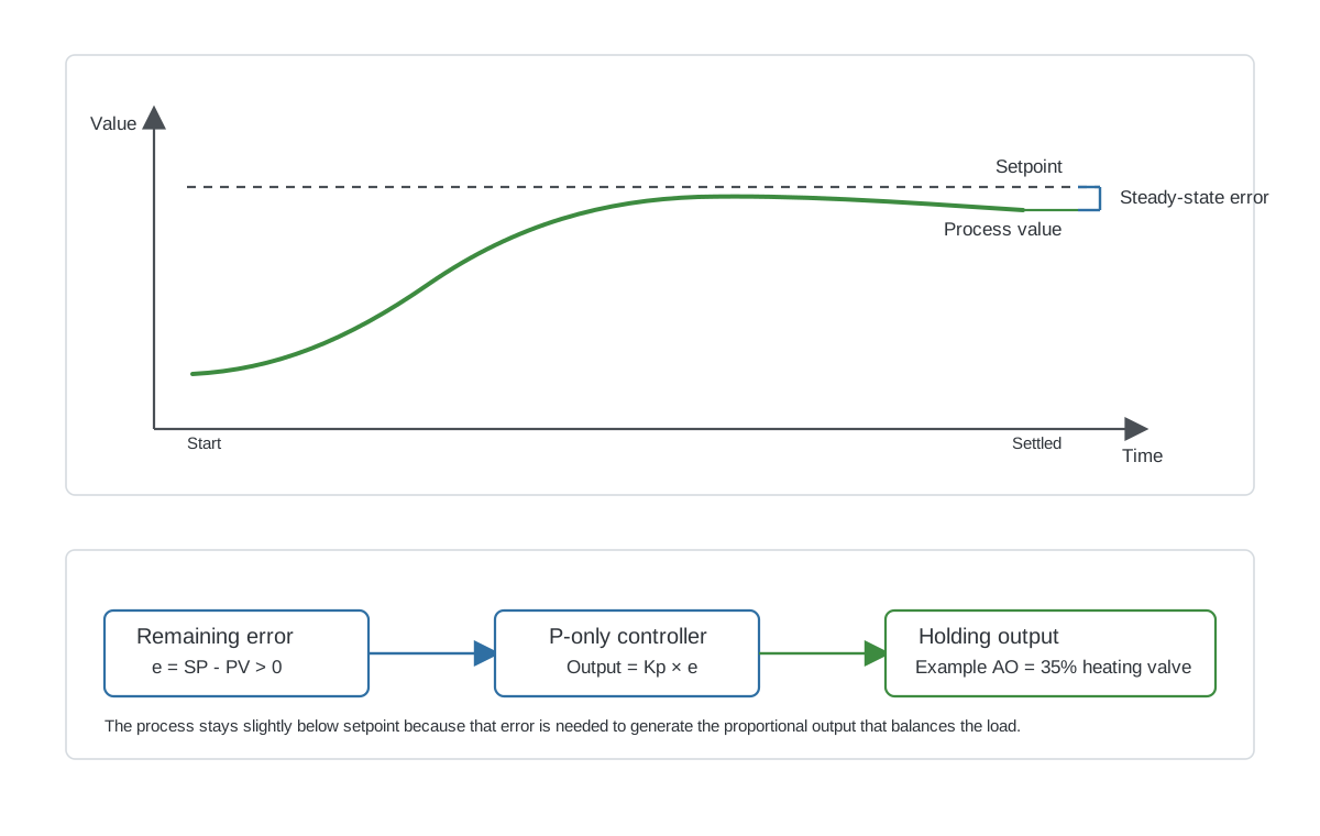
A proportional-only controller often needs a permanent error to produce the output required by the process. Consider a heating loop where the valve must remain 35% open to maintain the desired temperature. If the controller has no output bias and uses a 10 K proportional band, a 35% proportional output requires an error of 3.5 K. The process may therefore stabilize 3.5 K below the setpoint.
This is called steady-state error or offset. The loop can be completely stable and still remain away from the setpoint. Making the P-band smaller reduces the error required to create the same output, but excessive proportional action can make the loop unstable. The integral term solves this problem in a different way by building the required steady output over time.
5. Integral control: removing error that remains
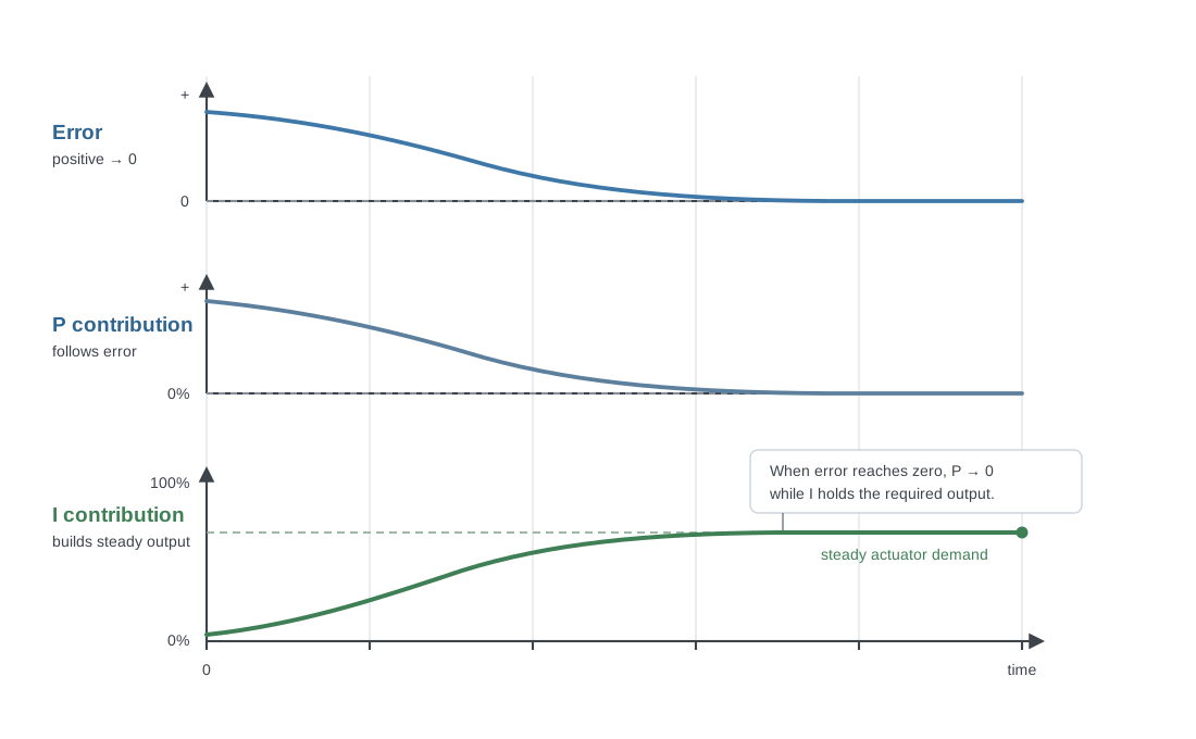
The integral term reacts to both the size of the error and how long the error has existed. If the process remains below the setpoint, the integral contribution keeps increasing. If the process remains above the setpoint, the integral contribution moves in the opposite direction. This allows a PI controller to build the steady output needed by the process even after the proportional error becomes almost zero.
Consider a heating loop that finally needs a 37% valve position to hold the setpoint. During warm-up, the proportional term may initially provide most of the output because the error is large. As the temperature approaches the setpoint, the proportional contribution becomes smaller. At the same time, the integral term has accumulated because the temperature spent time below the setpoint. Once the measurement reaches the setpoint, the proportional term may be close to zero while the integral term remains around the 37% required to hold the temperature.
This is why integral action eliminates the steady-state offset of proportional-only control. It also explains why integral tuning has to be matched to process speed. If integral action builds much faster than the physical system can respond, the controller can store too much output before it sees the result. The process then overshoots and the integral term has to unwind in the opposite direction.
5.1 Integral gain, integral time and 1/I are different parameter conventions
Integral action is one of the places where controller terminology causes the most confusion. A controller may expose integral gain Ki, integral time Ti, reset time, repeats per minute, or a reciprocal/divisor value. These parameters can describe the same physical action but move in opposite numerical directions.
With integral gain, a larger value means stronger integral action. With integral time Ti, a larger value normally means slower integral action because the controller takes longer to build the same contribution. A smaller integral time makes the integral term build faster. If a controller exposes a reciprocal coefficient such as 1/I, then a larger coefficient again means stronger integral action.
For the common ideal time form, the controller can be written conceptually as:
output = Kp x [ error + (1 / Ti) x accumulated error + Td x error rate ]
The integral coefficient is therefore proportional to Kp / Ti. This is why copying an integral time from one controller to an integral gain field in another controller gives meaningless tuning even when both fields are labelled with the letter I.
5.2 Integral windup
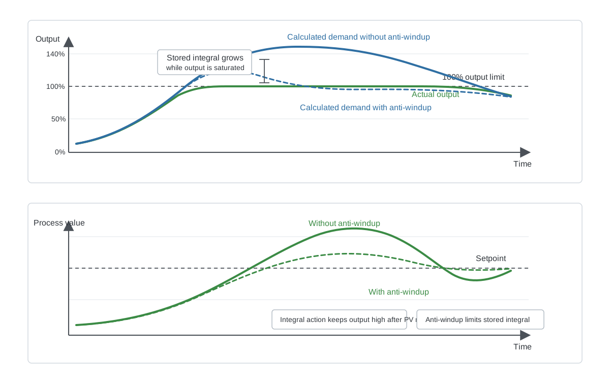
Integral windup happens when the integral term continues accumulating while the physical output is already at a limit. Imagine a heating loop during startup with a large positive error. The controller calculates 160% output, but the valve can only open to 100%. If the integral term continues increasing while the valve remains fully open, the internal controller demand may rise far above 100% even though the physical actuator cannot respond further.
When the temperature finally approaches the setpoint, the controller may still contain a large positive integral contribution. The valve remains at 100% longer than it should, the temperature overshoots, and the integral term then needs time to unwind. Modern PID implementations commonly include some form of anti-windup that stops or corrects integral accumulation when the output is saturated in a direction that cannot reduce the saturation.
Output saturation is not automatically a tuning problem. A heating valve reaching 100% during a cold start can be completely normal. The important question is how the integral calculation behaves while the output is limited and how quickly the loop recovers when the process comes back into controllable range.
6. Derivative control: reacting to the rate of change
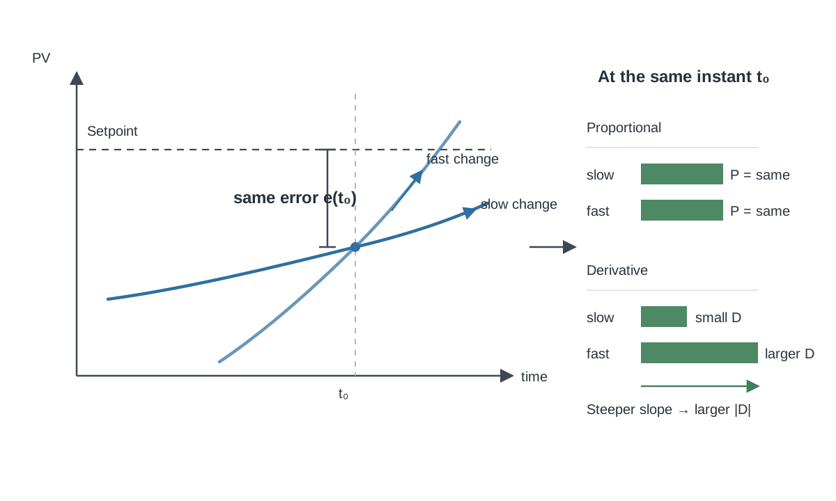
The derivative term reacts to how quickly the process error or measured value is changing. Two situations can have the same current error but very different dynamics. A temperature may be 2 K below setpoint and rising slowly, or it may be 2 K below setpoint and rising extremely quickly. Proportional action sees the same current error in both cases. Derivative action can distinguish the rate of change and reduce or increase the controller response before the process crosses the setpoint.
A well-tuned derivative term can add damping to a process and reduce overshoot. It can be useful when the process has enough predictable dynamic behavior for the rate of change to carry useful information. The problem is that derivative action also reacts strongly to measurement noise because noise is, by definition, a rapid change in the measured signal. A temperature input that moves between 20.00, 20.05, 19.98 and 20.04 °C can produce a much larger derivative response than the actual thermal process warrants.
For this reason, many HVAC loops use PI control. Temperature, humidity and room measurements are often slow enough that good proportional and integral tuning is sufficient. Duct pressure can be fast, but it may also contain fan and airflow noise. Full PID is not automatically better than PI. Derivative action should be added because the process benefits from it, not because the controller happens to have a D parameter.
Many practical controllers filter the derivative calculation. Some also calculate derivative action from the process value instead of the error so that a sudden setpoint change does not create a large derivative kick. These implementation details are another reason to verify the actual controller algorithm before transferring tuning values.
7. Understanding Kp, Ti, Td and the 1/P, 1/I, 1/D form
There is no single universal way to present PID tuning parameters. The most useful approach is to understand the equation behind the controller and then translate the parameters instead of trying to memorize manufacturer-specific labels.
A parallel gain form can be written as:
u = Kp x e + Ki x integral(e dt) + Kd x de/dt
Here u is the controller output, e is the error, and Kp, Ki and Kd are direct gains. Increasing any one of these gain values strengthens the corresponding P, I or D contribution.
A common time form is:
u = Kp x [ e + (1 / Ti) x integral(e dt) + Td x de/dt ]
In this form, Kp still strengthens proportional action when it is increased, but Ti behaves in the opposite direction because it is in the denominator. A larger Ti makes integral action slower. Td multiplies the derivative action, so a larger derivative time normally makes D stronger within this particular equation.
A controller can also be expressed in a reciprocal or divisor form:
u = e / P + integral(e dt) / I + (de/dt) / D
The same equation can be written as:
u = (1/P) x e + (1/I) x integral(e dt) + (1/D) x de/dt
This form directly shows the 1/P, 1/I and 1/D coefficients. When u is normalized from 0 to 1, P has the practical meaning of the process error required for a full-range proportional contribution. For example, P = 10 K means a 10 K error gives a proportional contribution of 1.0, or 100%. The proportional coefficient is 1/P = 0.1 1/K.
The equivalent coefficients between the ideal time form and the reciprocal form are:
1/P = Kp
1/I = Kp / Ti
1/D = Kp x Td
This means the divisor parameters are related by:
P = 1 / Kp
I = Ti / Kp = P x Ti
D = 1 / (Kp x Td) = P / Td
The important point is that a literal parameter called I in one controller is not necessarily the same quantity as Ti in another controller. The same warning applies even more strongly to D because derivative implementations often include filtering, derivative-on-measurement logic or other details. The interactive tuning simulator uses a proportional-band/time view internally and can display the mathematically equivalent 1/P, 1/I and 1/D coefficients used by its own equation. This makes the relationship visible without suggesting that every commercial controller uses exactly the same parameterization.
7.1 What 1/P means in percentage terms
For a normalized output, the proportional contribution is:
P contribution = error x (1/P)
For a 0 to 100% output, multiply that result by 100%. With a 10 K proportional band and a 2 K error:
1/P = 1/10 = 0.1 1/K
2 K x 0.1 1/K = 0.2
0.2 x 100% = 20%
This is the cleanest practical interpretation of proportional band. The error tells you how far through the band the process currently is. A 2 K error inside a 10 K band represents 20% of the full output range. A 5 K error represents 50%, and a 10 K error represents 100%.
8. P, PI and PID compared on the same process
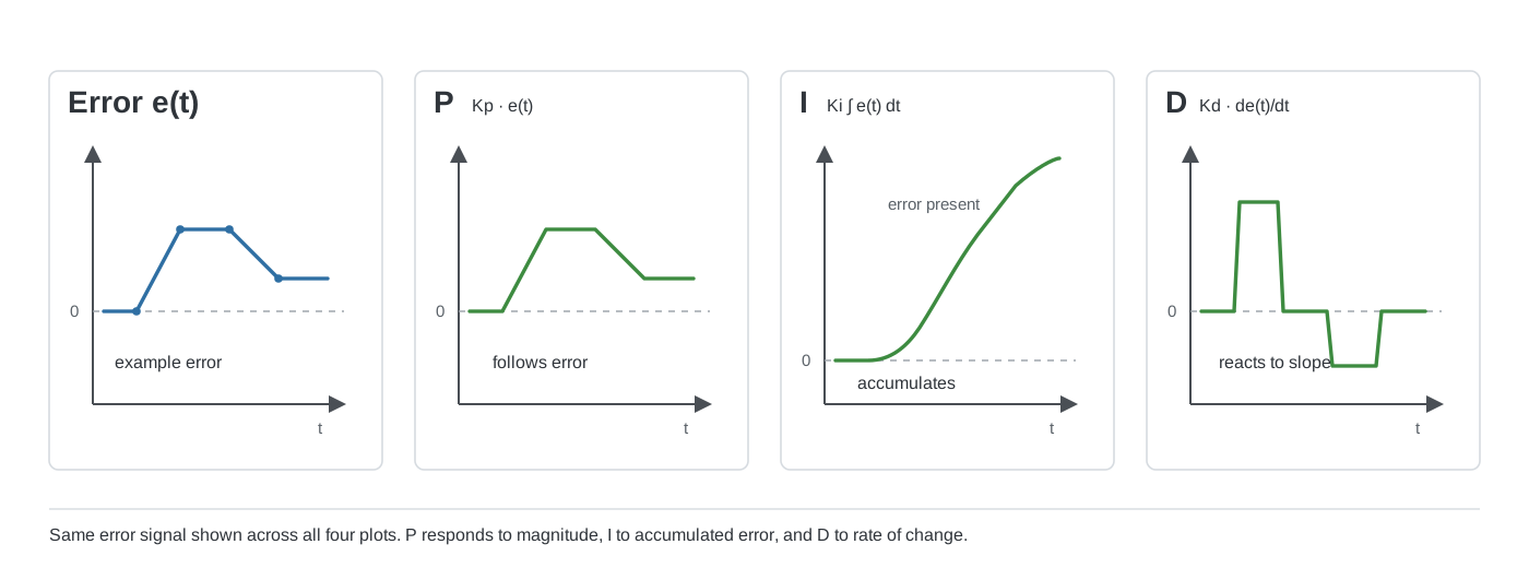
A P controller only reacts to the current error. It can be simple and stable, but it normally needs some error to create a steady output change after the load changes. A PI controller adds integral action and can therefore remove that remaining error. A PID controller adds derivative action, which can improve damping and responsiveness when the derivative signal is useful and the implementation is properly filtered.
The comparison below starts all three controllers at the same operating point and then adds the same load disturbance. The P controller settles with an offset because it needs a permanent error to create the extra output. The PI controller builds additional integral output and returns to the setpoint. The PID controller uses the same integral correction while derivative action changes the transient response.
The comparison should not be read as proof that PID is always faster or better. Different P, I and D values can produce very different results. The point is to show what each controller type is capable of doing and why PI is such a common choice in building automation.
9. The physical process determines the tuning
A PID controller is tuned to a process. There is no generally correct P-band or integral time that can be copied to every loop. The controller has to be matched to how strongly the process responds to output, how quickly it responds and how much delay exists before the measurement shows the result.
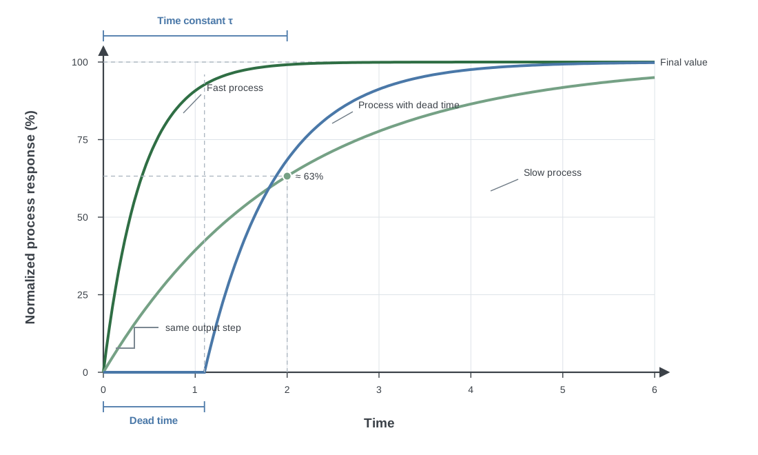
Process gain describes how much the measured value changes when controller output changes. A small valve movement may create a large supply temperature change if the valve is oversized. The same 10% output change may produce only a small effect in another system. Higher process gain normally requires a less aggressive controller because the physical system already amplifies output changes strongly.
Time constant describes the speed of the process response. Duct pressure can react within seconds after a fan speed change. Supply air temperature may react over tens of seconds. A room or concrete floor heating system may react over many minutes or hours. Integral action that is reasonable for a pressure loop can be far too fast for a room temperature loop.
Dead time is the delay before a controller action becomes visible in the measurement. A temperature sensor installed far downstream from a heating coil sees the effect only after the heated air travels through the duct. A sensor mounted inside a large pipe pocket has its own thermal response delay. Dead time makes control more difficult because the controller is acting while still seeing old process information.
10. How aggressive tuning becomes oscillation
A control loop oscillates when the controller repeatedly over-corrects the process. The controller raises the output because the measurement is low, but by the time the process responds the output has already been increased too far. The measurement crosses the setpoint, so the controller moves strongly in the opposite direction. If the same thing repeats, the loop hunts around the setpoint.
Too much proportional action is one common cause. With proportional-band tuning this means the P-band is too small. Integral action can also create oscillation when it accumulates faster than the process can respond. Process dead time makes both problems worse because the controller has to wait longer before it sees the consequence of its previous action.
A trend often gives better information than the parameter values themselves. A fast repeating oscillation can indicate overly strong proportional action in a fast process. A large slow oscillation often points toward integral action that is too aggressive for the process. An actuator continuously moving back and forth can also be caused by noisy measurement, excessive derivative action, an oversized valve, poor valve authority, backlash or a control loop fighting another control loop.
11. A practical manual tuning method for HVAC PI loops
For many HVAC loops, start by tuning a PI controller and leave derivative action disabled. The objective of the first step is to find proportional action that is strong enough to respond clearly but not so strong that the process continuously oscillates. Integral action can then be added to remove the remaining steady-state error.
Start with a relatively wide proportional band so the controller is deliberately mild. Disable integral and derivative action if the controller allows it. Make a controlled disturbance or a small setpoint change and watch the process trend. If the response is far too weak, reduce the proportional band in steps. Allow enough time after each change for the physical process to reveal the result. Do not change the parameter every few seconds when the process takes several minutes to respond.
Continue strengthening proportional action until the response is clearly useful. If the process begins to oscillate or the actuator moves too aggressively, increase the proportional band again. The goal is not to find the smallest possible P-band. The goal is to find a stable proportional response with enough authority to handle normal disturbances.
Then enable integral action with a slow setting. If the controller uses integral time, start with a larger time and reduce it gradually. If it uses integral gain or 1/I, start with a small coefficient and increase it gradually. Watch how quickly the remaining error disappears and whether the process overshoots. Integral action should correct a persistent error without becoming the main cause of oscillation.
After the loop works for a setpoint change, test a real load disturbance. Open dampers, change airflow, change water load, or use another safe operating change that represents what the system actually experiences. A controller that follows a setpoint ramp well may still reject disturbances poorly. Final tuning should be judged from normal operating behavior, not from one ideal test.
If derivative action is considered necessary, add it only after P and I are understood. Increase it gradually and watch measurement noise and actuator movement. If D makes the output noisy without improving the process response, remove it. PI is a complete controller and is often the better engineering choice for HVAC.
12. Tuning by symptoms
A trend can usually tell you which part of the loop needs attention. The table below is a starting point, not an automatic diagnosis. Mechanical problems, wrong sensor placement, actuator saturation and interacting control loops can produce symptoms that look like bad PID tuning.
| Observed behavior | Likely control issue | Typical direction to investigate |
|---|---|---|
| Loop reacts very slowly to a disturbance | Proportional action too weak | Reduce P-band or increase Kp |
| Fast sustained oscillation | Proportional action too strong | Increase P-band or reduce Kp |
| Stable but remains away from setpoint | No or insufficient integral action | Increase integral action |
| Large slow overshoot and recovery | Integral action too strong | Increase Ti or reduce Ki / 1/I |
| Large overshoot after long 100% output | Integral windup | Check anti-windup and saturation behavior |
| Output changes rapidly with noisy measurement | D or P too aggressive, insufficient filtering | Reduce derivative action, review P and filtering |
| Valve moves constantly while PV barely changes | Tuning, valve sizing, backlash or sensor noise | Check mechanics and process before retuning |
| Output stays at 0% or 100% | Process cannot reach setpoint, wrong direction or limits | Check capacity, action direction and output limits |
13. Output limits, deadband and anti-windup
The PID calculation may mathematically request any value, but real actuators have limits. A valve generally operates between 0 and 100%. A fan may have a configured minimum speed of 25% and maximum speed of 90%. A heating stage may only be allowed to operate between specific limits because of equipment requirements. The controller must respect these limits and its integral logic should understand when the actual output can no longer follow the internal demand.
Output limits also affect tuning. If a fan controller is tuned while it can operate from 0 to 100% and the minimum is later changed to 40%, the available control range and operating point have changed. If a valve spends most of its time close to 0% because it is oversized, small output changes may produce disproportionately large process changes. That is a process and valve-sizing issue, not something that should be hidden with extreme PID tuning.
A deadband can be used when tiny errors should not create continuous output movement. Inside the deadband the error is treated as zero or reduced according to the controller implementation. This can be useful with noisy measurements or actuators that should not move for every small fluctuation. Too much deadband, however, creates an intentional control error and can make the process look poorly regulated.
Anti-windup belongs in the same discussion because it connects the internal controller calculation to the physical output limits. A useful implementation prevents integral action from continuing to build in a direction that would push an already saturated output further beyond its limit. Some controllers freeze the integral, some back-calculate it from the saturated output, and some use other tracking methods.
14. Sampling time and execution interval
A digital controller does not calculate PID continuously. It runs the calculation at discrete intervals. A PLC program may execute the controller every 100 ms, every second, every 10 seconds or according to another task cycle. The integral and derivative terms depend directly on time, so the execution interval must be included in the calculation.
A simple integral implementation that repeatedly performs integral = integral + error is incomplete because the result changes if the program cycle changes. The time-aware form is conceptually integral = integral + error x dt, where dt is the time since the previous calculation. The derivative term similarly uses a rate such as (error_now - error_previous) / dt.
This matters when a PID function block is moved to a different task, when a PLC cycle time changes, or when someone writes a custom controller in Structured Text. A well-designed PID function block either receives the execution interval as a parameter or measures it internally. The tuning values and the algorithm have to use compatible time units.
Derivative action is especially sensitive to sampling because it calculates rapid changes between samples. Very short intervals can expose more measurement noise. Very long intervals can miss important dynamics. The control calculation should normally run substantially faster than the process dynamics it is trying to regulate.
15. Measurement filtering and sensor placement
PID quality is limited by measurement quality. A controller cannot distinguish real process movement from a bad sensor, electrical noise or unsuitable placement unless filtering and process knowledge make the difference clear. If a pressure transmitter produces a noisy signal, aggressive proportional or derivative tuning can turn that noise into continuous fan-speed movement.
Filtering can smooth a measurement before it enters the controller, but filtering also adds delay. Heavy filtering may make the trend look clean while making the control loop harder to tune because the controller is always reacting to an older value. The correct amount of filtering is enough to remove irrelevant high-frequency noise without hiding the actual process response.
Sensor placement can have an even larger effect. A supply air sensor too close to a heating coil may see strong local temperature variation. A sensor too far downstream may add transport delay. A pressure sensor mounted where airflow is turbulent can create unnecessary noise. A slow immersion sensor can add thermal lag. Before changing PID parameters, confirm that the measurement represents the process you actually want to control.
For more detail on sensor behavior, transmitter scaling, drift and placement, see the Building Automation Sensors and Transmitters guide.
16. Actuator behavior changes the loop
The controller output is only a request. The actuator still needs time to move and the controlled device needs to convert that movement into a physical effect. A fast 0 to 10 V valve actuator, a 180-second floating actuator and an electrothermal valve driven with pulses cannot be treated as identical final control elements even if the calculated PI demand is 50% in every case.
Valve sizing and authority matter as well. If most of the useful heating change happens between 0 and 20% valve command, the effective process gain is very high in that part of the stroke. The controller may appear too aggressive near closed position and too weak elsewhere. A nonlinear valve characteristic or badly balanced hydronic system can therefore create tuning behavior that cannot be solved perfectly with one set of linear PID parameters.
Variable frequency drives introduce their own dynamics. Minimum speed limits, acceleration ramps and fan pressure characteristics affect how quickly a pressure controller can change the process. If a fan has a long ramp time, the PI controller should not integrate aggressively while waiting for speed to catch up.
17. Continuous PI output to a 0 to 10 V actuator
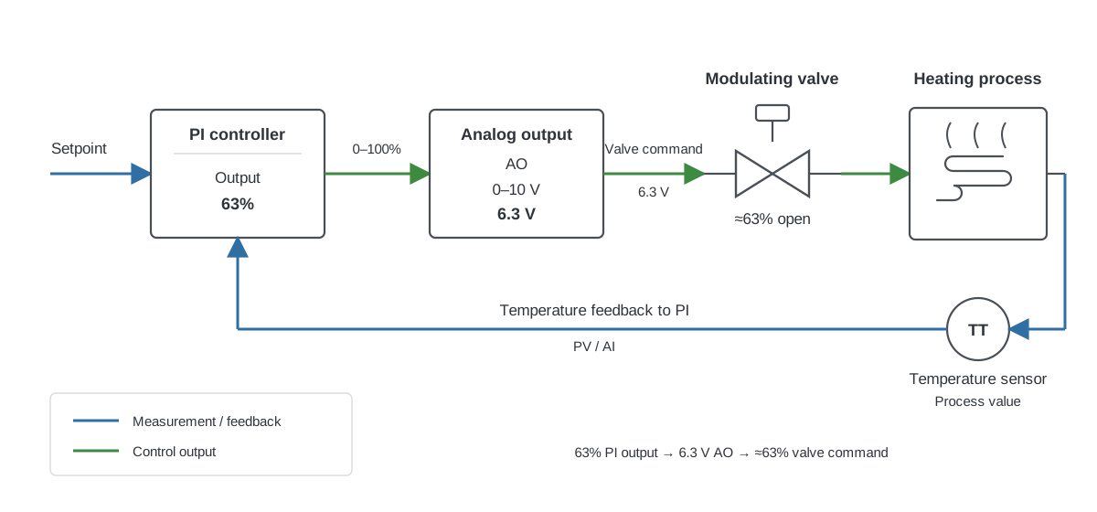
The simplest output case is a continuous modulating actuator. The PI controller calculates a value from 0 to 100%, and the analog output converts that percentage into the actuator signal. With a 0 to 10 V valve actuator, 63% controller output normally becomes approximately 6.3 V if the output is scaled linearly and has no special limits.
The control chain is therefore straightforward. The sensor produces the process value, the PI controller calculates the required demand, the analog output converts demand into voltage, and the actuator moves the valve. The valve movement changes the process, which is measured again on the next controller cycle.
SP 60.0 C
PV 57.2 C
      |
      v
PI controller = 63%
      |
      v
AO = 6.3 V
      |
      v
Valve approximately 63%
The BMS I/O guide explains analog outputs, 0 to 10 V signals and actuator interfaces in more detail.
18. PI control with a pulse output
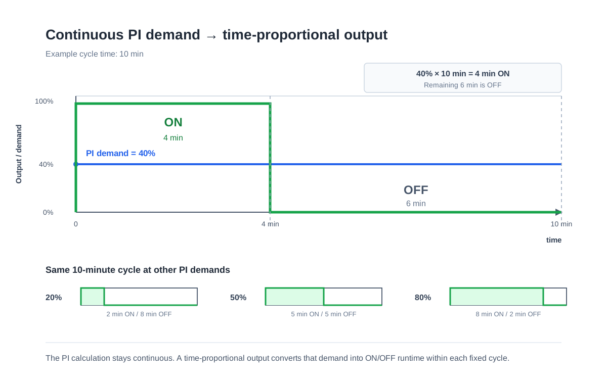
A PI controller does not require a physically analog output. The controller can calculate a continuous demand from 0 to 100% and then convert that demand into time-proportional switching. This is useful when the final device only supports on/off control but the controlled process is slow enough to average the pulses over time.
Consider a hydronic room-heating zone with an electrothermal valve actuator. The PI controller may calculate 40% heating demand even though the actuator input is only ON or OFF. With a 10-minute pulse period, the output can be ON for 4 minutes and OFF for 6 minutes. A 75% demand becomes 7.5 minutes ON and 2.5 minutes OFF. The room and water system are slow enough that the heat output is averaged over many cycles.
The cycle period has to suit the actuator and process. A mechanical or thermal actuator should not be switched faster than it can physically respond or faster than its manufacturer permits. A very long period gives coarse control because the process receives large blocks of heating and no heating. A very short period may create unnecessary switching without improving the actual room response.
The pulse simulator runs faster than real time so that a multi-minute heating cycle can be observed in seconds. The PI controller still calculates a continuous demand. The time-proportional stage then compares that demand with the position inside the current cycle and switches the heating valve ON for the required fraction of the cycle.
19. Time-proportional output is not the same as floating control
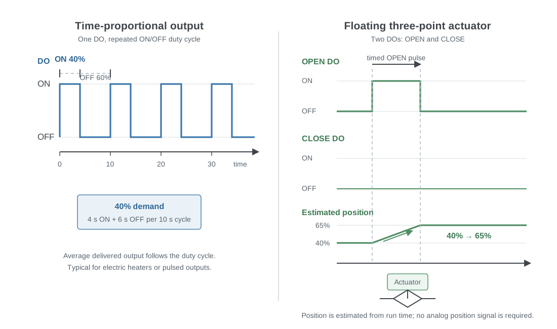
Time-proportional switching and floating three-point actuator control both use digital outputs, but they solve different problems. A time-proportional output represents a power or demand percentage over time. A 40% demand means the output is ON for approximately 40% of the configured period.
A floating actuator has separate OPEN and CLOSE commands and a known or estimated travel time. If a 120-second valve actuator is believed to be at 40% position and the controller wants 65%, the control logic may drive the OPEN output for roughly 30 seconds to move 25% of full travel. It then stops both outputs. The control logic is trying to estimate or track actuator position, not create a 40% duty cycle.
This distinction is important when designing outputs. A thermal on/off valve can be well suited to time-proportional control. A three-point mixing valve needs open/close movement logic. A 0 to 10 V actuator accepts a continuous analog command directly. The same PI demand can therefore require very different output handling depending on the final actuator.
20. Heating water temperature example
A heating water temperature loop is a useful example because the relationship between measurement, valve and load is easy to follow. Assume the supply temperature setpoint is 60 °C. A temperature sensor measures 54 °C, so the heating error is +6 K. The PI controller increases the valve command and more heat is transferred to the water.
As the temperature rises, proportional action becomes smaller because the error is shrinking. Integral action continues to adjust until the output is exactly what the current load requires. If the building load increases and return water becomes colder, the supply temperature begins to fall. The proportional term reacts immediately to the new error, while integral action changes more gradually until the new steady valve position has been found.
The correct tuning depends on water volume, flow rate, valve authority, heat exchanger capacity, sensor response and transport delay. A small local heating circuit can react quickly. A large circuit with a sensor far from the valve can react much more slowly. The controller should be tuned from the measured process response, not from a generic temperature-loop number.
21. Supply air temperature example
Supply air temperature is one of the most common PI loops in an air handling unit. The controller compares measured supply temperature with its setpoint and adjusts heat recovery, heating and cooling according to the control sequence. In a simple heating-only case, a low supply temperature increases heating valve demand and a high temperature reduces it.
The process can contain several delays. The valve has an actuator runtime, water flow through the heating coil changes heat transfer, the air needs time to travel from the coil to the temperature sensor, and the sensor itself has a response time. If the supply sensor is placed far downstream, controller action may not appear in the measurement immediately. Aggressive integral action during this delay can create repeated overshoot.
An AHU may also use staged control, for example heat recovery first, then heating, then cooling in another direction. The main PI demand can still be continuous, but the sequence converts that demand into several physical outputs. The Interactive AHU Simulator demonstrates supply temperature and pressure regulation in a complete air handling process.
22. Duct pressure example
A duct pressure loop is usually much faster than a room temperature loop. The pressure transmitter measures static pressure and the PI controller changes fan speed through a VFD. When dampers open, system resistance changes and duct pressure tends to fall. The controller increases fan speed to restore pressure.
Because the process responds quickly, the control interval and tuning can also be faster. At the same time, pressure signals may contain turbulence and fan-related fluctuations. If the proportional gain is too high, the fan speed hunts. If integral action is too fast, the fan can repeatedly overshoot the required pressure. If derivative action is used without suitable filtering, small pressure fluctuations can create unnecessary output movement.
A badly selected pressure sensor range also affects control resolution. A 0 to 2500 Pa transmitter used for a 200 Pa duct setpoint provides much less useful signal resolution than a correctly selected range. PID tuning cannot recover information that the measurement chain does not provide.
23. Room heating example
Room temperature is a slow process with large and changing disturbances. Outdoor temperature, solar gain, occupancy, doors, windows and internal equipment all change the heating load. The heating emitter and building mass add further delay. A room may therefore need integral times measured in many minutes rather than seconds.
A PI controller is normally a natural choice. Proportional action changes heating demand according to the current room error. Integral action slowly corrects the remaining error caused by the steady heat loss. If a pulsed thermal actuator is used, the continuous PI demand is converted into a duty cycle as shown earlier.
Fast tuning is usually harmful in this type of loop because the controller cannot force the room to respond faster than the building physics allow. If integral action increases strongly during a long warm-up, stored demand can create overshoot hours later. Output limiting, anti-windup, suitable room sensor placement and realistic setpoint scheduling are often more important than adding derivative action.
24. Cascade control
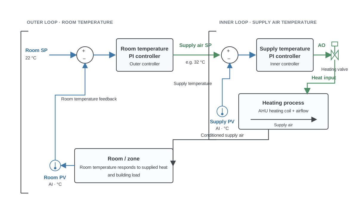
Cascade control uses one controller to generate the setpoint for another controller. A common HVAC example is room temperature control through a supply air temperature setpoint. The outer room controller does not directly move the heating valve. Instead, it adjusts the supply temperature target. The inner supply temperature PI controller then moves the valve to achieve that target.
The inner loop should normally be faster than the outer loop. Supply air temperature can change much faster than room temperature, so this relationship is natural. The inner controller handles fast disturbances in the air-handling process while the outer controller slowly adjusts how much heating or cooling the room needs.
Poor cascade tuning can create loops that fight each other. If the outer loop changes its setpoint faster than the inner loop can follow, both controller integrals may build at the same time and produce unnecessary oscillation. Tune and verify the inner loop first, then tune the slower outer loop around it.
25. Setpoint reset and compensation are separate from PID
The setpoint supplied to a PID controller does not have to be constant. Building automation often calculates the setpoint from another condition. A heating water supply setpoint may rise when outdoor temperature falls. A duct pressure setpoint may reset according to terminal damper positions. A supply temperature target may be adjusted from room demand.
This reset logic should be kept conceptually separate from the PID calculation. The reset function decides what setpoint is required. The PI or PID controller decides what actuator output is required to reach that setpoint. Mixing these two functions together makes troubleshooting harder because a moving setpoint can look like unstable control when it is actually being commanded by supervisory logic.
When testing a PID loop, trend both the setpoint and measured value. A process value that appears to wander may actually be tracking a setpoint that is being reset continuously.
26. Common PID commissioning mistakes
One common mistake is tuning before verifying the physical loop. A wrong sensor, reversed valve, closed isolation valve, incorrectly scaled analog output or saturated actuator must be fixed before PID tuning starts. Otherwise the controller is being adjusted to compensate for a fault.
Another mistake is confusing proportional gain with proportional band. Increasing Kp makes a controller stronger, while increasing proportional band makes it weaker. The same problem appears with integral parameters. Increasing integral gain makes integration stronger, while increasing integral time makes it slower. A parameter called simply I cannot be interpreted safely without its unit and algorithm.
Changing several tuning parameters at once also makes the result difficult to understand. If P-band, integral time and output limits are all changed together, the next trend cannot tell you which change improved or damaged the response. Make one meaningful change, wait for the process, and compare the result.
Tuning faster than the process can respond is especially common in HVAC. A technician changes the integral time, watches the trend for 20 seconds, sees little change and adjusts it again even though the physical loop has a five-minute response. By the time the process catches up, the tuning may have been changed several times and integral action is already excessive.
Another mistake is adding D because the controller is called PID. A stable PI loop that reaches setpoint and rejects disturbances does not need derivative action. D should solve a specific dynamic problem. If it only makes the output noisier, it is not improving control.
27. Commissioning checklist before tuning
Before tuning the controller, confirm that the process can actually be controlled. The measurement should be correctly scaled and believable. The actuator should move through the required range and in the correct direction. Output limits should match the equipment. The setpoint should be physically achievable under the current load. Any interlocks, minimum positions, staging logic and manual overrides should be understood before interpreting the PID trend.
During tuning, trend at least the setpoint, process value and controller output. If possible, also trend the physical actuator feedback or a value that represents the actual process load. Make one change at a time and wait long enough to see the process response. Test a representative disturbance in addition to a setpoint change.
After tuning, check operation at more than one load condition. A loop that works at mild outdoor temperature may behave differently at design heating load. Check whether the actuator spends long periods at 0% or 100%, whether the integral recovers cleanly from saturation, whether the output moves continuously because of noise, and whether the process remains stable when supervisory setpoints change.
28. Key points to remember
The proportional term reacts to the error that exists now. Integral action reacts to accumulated error and is what normally removes steady-state offset. Derivative action reacts to rate of change and can add damping, but it is often unnecessary in slow or noisy HVAC loops.
When the controller uses proportional band, a smaller P-band means stronger proportional action. For a normalized controller, P contribution = error / P-band, so a 2 K error inside a 10 K band creates a 20% proportional contribution. This is the practical meaning of the 1/P relationship.
Parameter conventions must always be checked. Kp, proportional band, Ti, Ki, Td, Kd, 1/P, 1/I and 1/D can describe related controller behavior but they are not interchangeable labels. Translate the actual equation and units before copying tuning values.
The physical process sets the limits of good control. Sensor delay, actuator speed, valve sizing, process gain, time constant, dead time, output limits and disturbances all affect the trend. A PID parameter should be changed only after the rest of the loop has been checked.
For many building automation processes, a well-tuned PI controller is the correct solution. Start simple, observe the process, tune proportional action first, add integral action gradually, and use derivative action only when the process gives a clear reason for it.
Frequently asked questions
Is PID always better than PI?
No. PI control is sufficient for many HVAC processes because proportional action provides the immediate response and integral action removes the remaining error. Derivative action can improve some dynamic responses, but it can also react strongly to measurement noise and add tuning complexity. Use D when it improves a specific process response.
What does proportional band mean?
Proportional band is the change in process value that produces a full-range proportional output change. If the P-band is 10 K, a 10 K error corresponds to 100% proportional contribution, a 5 K error to 50%, and a 1 K error to 10%, assuming a normalized linear controller without other scaling.
Is 1/P the proportional gain?
In the normalized proportional-band form, yes. If P is the proportional band, the coefficient multiplying error is 1/P. For a 0 to 100% output, the proportional contribution is error / P x 100%. A controller that uses a different PID form may define its P parameter differently, so the documentation still has to be checked.
Why does increasing proportional band make control slower?
A larger proportional band means the same error creates a smaller proportional contribution. If the error is 2 K, a 5 K band gives 40% while a 20 K band gives only 10%. The wider band therefore makes the controller less aggressive.
Why does a P controller stay away from the setpoint?
A P-only controller may need a permanent error to create the actuator output required by the process. Integral action can store the required steady output while allowing the error to return toward zero.
What is a good starting point for PID values?
There is no universal starting value because tuning depends on process gain, response speed, dead time, actuator behavior and controller parameter convention. For HVAC commissioning, a practical method is to start with mild proportional action, verify the response, strengthen it gradually, then add slow integral action and tune from the measured trend.
Can a PI controller drive a digital output?
Yes. The PI controller can calculate a continuous 0 to 100% demand and a separate time-proportional stage can convert that demand into an ON/OFF duty cycle. This is common with slow thermal processes and suitable binary actuators. The pulse period must match the actuator and process.
Why is my PID output always 100%?
The error may genuinely require full output, but constant saturation can also indicate wrong controller direction, insufficient equipment capacity, an unreachable setpoint, a sensor problem, incorrect scaling or excessive integral windup. Verify the complete control loop before changing tuning values.
Technical references
The explanations in this guide follow standard PID relationships and practical HVAC controller behavior. Manufacturer documentation is still required for the exact controller being commissioned because proportional band units, integral definitions, derivative filtering, output limiting and anti-windup behavior vary between implementations.